
Introduction
In the current post, we present the results of three different simulation methods for the same wind tunnel test, two of which are of significantly higher fidelity than the previous post. In addition, we assess the accuracy of the methods for predicting the flow. The first simulation is the traditional Reynolds Averaged Navier-Stokes (RANS) method. RANS is a steady state method that averages turbulence in time and models the smallest turbulence scales so that they do not have to be resolved through mesh discretization. The second method is Scale Adaptive Simulation (SAS). SAS is a variant of unsteady RANS where the Von Karman length-scale has been included allowing the solver to resolve eddies similar to Large Eddy Simulation (LES). The last method is DES, which is a combination of RANS and LES. DES uses RANS in regions where turbulence scales are small (such as near walls) and LES in the rest of the fluid domain. Both DES and SAS are transient methods. All of the methods utilize the Shear Stress Transport (SST) turbulence model.
Simulation Meshes
.png) |
| (a) |
.png) |
| (b) |
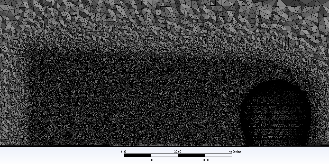.png) |
| (c) Figure 1: (a) Mesh for RANS model. (b) Mesh for DES and SAS models. (c) Cross sectional view of DES and SAS mesh scoped to the wake zone around the radome. |
Vortex Structures
Results of the RANS simulation are shown in Figure 2 and Figure 3. In both figures the results are mirrored about the symmetry plane to provide a complete picture. The pressure distribution on the radome is shown along with an iso-surface of the swirl strength around the radome. This surface is colored based on the flow velocity. One half is also semi-transparent to reveal the radome surface pressure contours and flow streamlines. The iso-surface is an indication of the presence of vortices. We see two major types of vortices in the flow. The first is horseshoe shaped and arcs around the front and sides of the radome. Behind the radome are a set of long wake vortices. These are formed as the flow separates on the backside of the radome. They are then turned and lengthened as the flow rolls them against the ground. |
Figure 2:
RANS simulation results. Close-up
view.
|
 |
Figure 3:
RANS simulation results. Broad
view.
|
Video 1 shows the transient response that is predicted using the SAS model. The motion has been slowed by roughly a factor of 30. As before, vortices around the radome are represented using swirl strength iso-surfaces, colored by the velocity magnitude. We see that the flow is much richer than predicted using RANS. The location of flow separation on the radome wanders with time and tightly wound vortices shed rapidly from the radome. They then roll over one another and coalesce into larger vortices that spread outward and continue to roll downstream. As they move they change shape, spinning off and consuming smaller vortices in a chaotic fashion. We note that the path of the vortices roughly matches that of the tubular vortices from the RANS model.
Video 2 shows the predicted response of the DES model. As with the SAS model, time is slowed by a factor of roughly 30. While the flow characteristics are still rich, the structure of the vortices is less chaotic. Larger, more stable vortices are shed from the radome surface. They combine quickly to form vortices that tend to hold their structure better as they grow and roll downstream.
Error Comparison
D’Amato and Fanning measured the time-averaged pressure at
over 200 points on the radome surface during their wind tunnel test. From this they determined the overall lift
and drag forces. Table 1
lists the measured data as well as the predicted values from three
simulations. The table also shows the
errors in the maximum and minimum pressures from the simulations, the root mean
squares (RMS) of their errors, as well as the lift and drag errors. We see that the method with the lowest error
is DES. It achieves RMS and lift errors
of 5.4% and 1.7%, respectively, which are roughly half that of the RANS
method. Unfortunately, none of the
methods predict the drag force well.
 |
| Table 1: Radome and simulation data and error. |
 |
Figure 4:
Plots of pressure error for RANS (left), SAS (middle) and DES (right)
solutions
|
Reference 1: D’Amato, R., Fanning, W. R., “Pressure Distributions on Sphere-Cone Radomes in Uniform and Gradient Flows,” Techincal Note, ESD-TR-68-84, Lincoln Library, MIT, 1968.


